Nucleus segmentation to SpatialData zarr#
spatialrefinery.segmentation segments nuclei in an H&E whole-slide image and packages the result as a SpatialData zarr store. It is two functions and a cells.geojson between them: segment_wsi runs InstanSeg over the slide, and geojson_to_spatialdata turns its polygons into a zarr carrying the slide image, the nucleus boundaries, and a table annotating them.
InstanSeg owns the whole-slide layer this needs – tiling, cross-tile label matching, an Otsu tissue prefilter so background is never segmented, and GeoJSON export. The GeoJSON in between is a resume boundary: a failed conversion does not force re-segmentation.
The table the conversion writes is all-zero counts over a template’s var. Nucleus segmentation produces no expression data, so the table exists to give the shapes element a SpatialData-valid annotation – and to fix the gene axis that inferred expression will later be written into.
This picks up where Converting images to OME-TIFF leaves off: the .ome.tif written there is exactly what segment_wsi reads. Segmentation needs the optional segmentation extra, which pulls instanseg-torch and therefore torch’s multi-GB CUDA wheels:
pip install "spatialrefinery[segmentation] @ git+https://github.com/peng-lab/spatialrefinery.git"
What you need: one TIFF-backed slide (.ome.tif, .svs, .ndpi, …), a template .h5ad whose var defines the gene axis, and a CUDA GPU. Runtime: on the 867 MB kidney H&E below, 8 minutes for segmentation (1239 tiles) and about a minute to write the zarr; CPU-only is possible but far slower.
from pathlib import Path

import spatialdata as sd
import spatialdata_plot  # noqa: F401 - registers the `.pl` accessor on SpatialData

from spatialrefinery.segmentation.instanseg import segment_wsi
from spatialrefinery.segmentation.to_spatialdata import default_zarr_path, geojson_to_spatialdata
Parameters#
SEG_OUTDIR holds the per-slide segmentation results and ZARR_OUTDIR the SpatialData stores. They are kept apart deliberately: the GeoJSON stage is the expensive one, so it is worth preserving independently of any zarr you rebuild from it.
TEMPLATE_ADATA is an AnnData whose var is the gene panel you intend to infer expression for. Only var is read – X, obs and everything else are ignored – so a panel definition saved from any matching study works.
WSI_PATH = Path(
    "/p/project1/hai_spatial_clip/data/phoenix_datasets/panels/multi_tissue/TENX/"
    "Xenium_V1_hKidney_nondiseased_section/Xenium_V1_hKidney_nondiseased_section_he_image.ome.tif"
)
SEG_OUTDIR = Path("/p/scratch/hai_1240/segmentation_files/segmentation_docs")
ZARR_OUTDIR = Path("/p/scratch/hai_1240/segmentation_files")
TEMPLATE_ADATA = Path("/p/scratch/hai_1240/segmentation_files/template_kidney_panel.h5ad")

SEG_OUTDIR.mkdir(parents=True, exist_ok=True)
ZARR_OUTDIR.mkdir(parents=True, exist_ok=True)
Step 1 – segment nuclei#
segment_wsi writes <outdir>/<slide filename>/cells.geojson. The directory keeps the full filename, extension included, so that a.svs and a.ndpi cannot land on top of each other. skip_existing=True (the default) returns immediately when that file is already there, which makes an interrupted batch resumable.
Two parameters are worth knowing before a first run:
pixel_size– microns per pixel, read from the slide metadata when omitted. InstanSeg rejects anything outside [0.1, 1] micron, so pass it explicitly for slides whose resolution tags are missing or nonsensical. The slide here reports 0.2738, so it is left out.clahe_clip/seed_threshold– InstanSeg normalises each tile by percentiles, so on weakly haematoxylin-stained slides pale nuclei fall below the seed threshold and are missed. Running CLAHE over each tile lifts local contrast (applied to L in LAB, so the H&E hue balance the model was trained on is preserved), and a lower seed threshold detects fainter nuclei. On this pale kidney section the two together found 83,554 nuclei against 67,168 at the defaults, +24.4%, with boundaries that hold up on visual inspection. Both are off by default; the values below are a reasonable start.
gpu_id is the CUDA device index, or None to force CPU.
geojson_path = segment_wsi(
    WSI_PATH,
    SEG_OUTDIR,
    gpu_id=0,
    clahe_clip=2.0,
    seed_threshold=0.4,
)
geojson_path
INFO     Segmenting Xenium_V1_hKidney_nondiseased_section_he_image.ome.tif with InstanSeg(brightfield_nuclei) on
         cuda:0
Model brightfield_nuclei version 0.1.1 already downloaded in /p/project1/hai_1240/spatialrefinery/.venv/lib/python3.12/site-packages/instanseg/utils/../bioimageio_models/, loading
INFO     Applying CLAHE (clip=2.0) to each tile before inference
Exporting to geojson
INFO     Wrote
         /p/scratch/hai_1240/segmentation_files/segmentation_docs/Xenium_V1_hKidney_nondiseased_section_he_image.om
         e.tif/cells.geojson
PosixPath('/p/scratch/hai_1240/segmentation_files/segmentation_docs/Xenium_V1_hKidney_nondiseased_section_he_image.ome.tif/cells.geojson')
Step 2 – build the SpatialData zarr#
geojson_to_spatialdata assembles three elements:
images["he_image"]– a lazy multiscale image built straight from the slide’s own pyramid throughtifffile’s zarr interface, so dask reads only the blocks a write touches. A level-0 plane on this slide is 33427 x 11949 x 3, about 1.1 GiB if it were materialised.shapes["nucleus_boundaries"]– one polygon per nucleus, in pixel coordinates.tables["table"]– all-zero counts overTEMPLATE_ADATA’svar, annotating the shapes, with nucleus centroids inobsm["spatial"].
default_zarr_path gives the store its conventional name: the slide’s stem plus .zarr, so Xenium_..._he_image.ome.tif becomes Xenium_..._he_image.zarr. The whole extension goes, which Path.stem alone would not do – it strips only the last suffix and would leave ...he_image.ome. Note this differs from step 1, whose directory keeps the full filename.
write_zip=True (the default) also writes an uncompressed <name>.zarr.zip beside the store. A zarr is tens of thousands of small files; the archive is what you actually move between filesystems.
The function also returns the object it just wrote, but its image element is still backed by the slide’s own TIFF rather than by the zarr. Read the store back from disk instead, as the next cell does – that is what any downstream consumer sees.
zarr_path = default_zarr_path(WSI_PATH, ZARR_OUTDIR)
print(zarr_path)

geojson_to_spatialdata(
    geojson_path=geojson_path,
    zarr_path=zarr_path,
    image_path=WSI_PATH,
    template_adata_path=TEMPLATE_ADATA,
)
print(f"wrote {zarr_path.name} and {zarr_path.name}.zip")
/p/scratch/hai_1240/segmentation_files/Xenium_V1_hKidney_nondiseased_section_he_image.zarr
INFO     Exploding multi-polygons from
         /p/scratch/hai_1240/segmentation_files/segmentation_docs/Xenium_V1_hKidney_nondiseased_section_he_image.om
         e.tif/cells.geojson
INFO     Reading exploded GeoJSON
INFO     Loading template AnnData: /p/scratch/hai_1240/segmentation_files/template_kidney_panel.h5ad
INFO     Building SpatialData object (83554 nuclei)
INFO     Writing SpatialData zarr to
         /p/scratch/hai_1240/segmentation_files/Xenium_V1_hKidney_nondiseased_section_he_image.zarr
INFO     Creating uncompressed zip archive
wrote Xenium_V1_hKidney_nondiseased_section_he_image.zarr and Xenium_V1_hKidney_nondiseased_section_he_image.zarr.zip
Inspect the result#
Read the store back from disk – the same thing any downstream consumer sees.
sdata = sd.read_zarr(zarr_path)
print(f"{len(sdata['nucleus_boundaries']):,} nuclei over a {sdata['table'].shape[1]}-gene panel")
sdata
83,554 nuclei over a 377-gene panel
SpatialData object, with associated Zarr store: /p/scratch/hai_1240/segmentation_files/Xenium_V1_hKidney_nondiseased_section_he_image.zarr
├── Images
│     └── 'he_image': DataTree[cyx] (3, 33427, 11949), (3, 16713, 5974), (3, 8356, 2987), (3, 4178, 1493), (3, 2089, 746)
├── Shapes
│     └── 'nucleus_boundaries': GeoDataFrame shape: (83554, 1) (2D shapes)
└── Tables
      └── 'table': AnnData (83554, 377)
with coordinate systems:
    ▸ 'global', with elements:
        he_image (Images), nucleus_boundaries (Shapes)
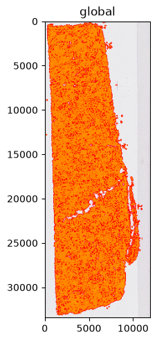
At full-slide zoom the nuclei are subpixel, so the overlay reads as tissue-shaped coverage: useful for checking that the Otsu prefilter kept to the tissue and did not wander into background.
sdata.pl.render_images("he_image").pl.render_shapes(
    "nucleus_boundaries",
    color="yellow",
    fill_alpha=0.7,
    outline_width=1.0,
    outline_alpha=1.0,
    outline_color="red",
).pl.show()
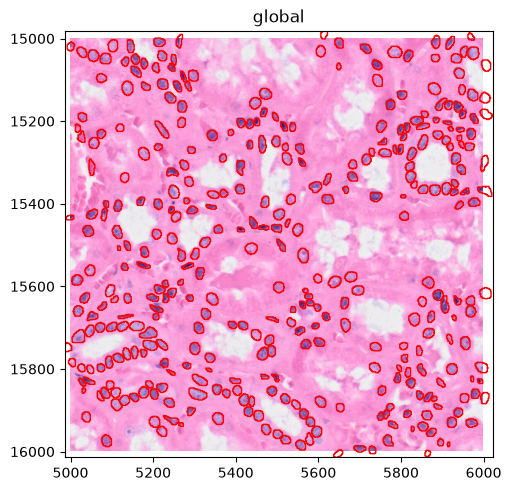
Individual boundaries only become visible on a crop. query.bounding_box subsets every element at once, in pixel coordinates on the "global" system.
cropped = sdata.query.bounding_box(
    axes=["x", "y"],
    min_coordinate=[5000, 15000],
    max_coordinate=[6000, 16000],
    target_coordinate_system="global",
)

cropped.pl.render_images("he_image").pl.render_shapes(
    "nucleus_boundaries",
    fill_alpha=0.0,
    outline_width=1.0,
    outline_alpha=1.0,
    outline_color="red",
).pl.show()
Expected output structure#
segmentation_docs/
└── Xenium_V1_hKidney_nondiseased_section_he_image.ome.tif/   # full filename
    └── cells.geojson

Xenium_V1_hKidney_nondiseased_section_he_image.zarr/          # stem only
├── images/he_image/          # multiscale, 5 pyramid levels
├── shapes/nucleus_boundaries/
├── tables/table/
└── zmetadata
Xenium_V1_hKidney_nondiseased_section_he_image.zarr.zip
Batch processing multiple slides#
Both stages skip work that is already on disk, so the loop below is safe to re-run over a directory: it picks up where an interrupted batch stopped rather than re-segmenting everything.
WSI_DIR = Path("ometiff_output")
written: list[Path] = []

for wsi in sorted(WSI_DIR.glob("*.ome.tif")):
    zarr_out = default_zarr_path(wsi, ZARR_OUTDIR)
    if zarr_out.exists():
        print(f"Skipping {wsi.name}: {zarr_out.name} already exists")
        continue

    try:
        cells = segment_wsi(wsi, SEG_OUTDIR, gpu_id=0, clahe_clip=2.0, seed_threshold=0.4)
        geojson_to_spatialdata(
            geojson_path=cells,
            zarr_path=zarr_out,
            image_path=wsi,
            template_adata_path=TEMPLATE_ADATA,
        )
    except Exception as e:  # noqa: BLE001 - one slide's failure must not abort the batch
        print(f"Failed on {wsi.name}: {e}")
        continue

    written.append(zarr_out)

print(f"Wrote {len(written)} SpatialData store(s)")
Wrote 0 SpatialData store(s)
Running this as a script#
The two stages have one CLI wrapper each, split on the same cells.geojson boundary. instanseg_segment.py prints GEOJSON_PATH=<path> and geojson_to_spatialdata.py prints ZARR_PATH=<path>, so they chain in a shell:
python scripts/instanseg_segment.py \
    --wsi-path slide.ome.tif \
    --outdir segmentation/ \
    --gpu-id 0 \
    --clahe 2.0 \
    --seed-threshold 0.4

python scripts/geojson_to_spatialdata.py \
    --geojson-path segmentation/slide.ome.tif/cells.geojson \
    --zarr-outdir zarrs/ \
    --wsi-path slide.ome.tif \
    --template-adata template.h5ad
What’s next#
That’s the full pipeline – see the API reference for the complete parameter list of each function used across these tutorials.